How to create a leave tracker in Excel

Keeping accurate leave records for employees is important not only to prevent disputes but also to ensure payroll accuracy, and facilitate effective workforce planning.

For small teams, an employee leave tracker in Excel is one easy way you can use to track your team’s PTOs. Excel allows you to organize leave data efficiently and use formulas to automate calculations, making it a powerful yet simple tool. Let’s see how you can build a simple employee leave tracker in Excel.

Step-by-step guide to creating a basic employee leave tracker in Excel

Here is a quick video walkthrough of how to create a leave tracker in Excel:

Step 1: Plan what you want in your leave tracker.

The best way to start building your leave tracker in Excel is to first have a plan in place. Think about:

1.Will each sheet feature a weekly or monthly tracker?
2.How much employee information are you going to add?
3.Do you want a tracker that only tracks absences, or do you also want to track other related details, such as overtime, work hours, or PTO accruals?

Once you have jotted down all that you want, give it a shape on paper. Chalk out the draft of the email tracker with everything that you want in it. Write details about what functionality or formula you are going to use on Excel to obtain a leave tracker as per your preferences.

We have figured that we are going to be creating a simple leave tracker in Excel today. This will include basic employee details, the leave types as per our company, the start and end dates of leave, the leave status, and the days of leave requested. So, let’s get started.

Step 2: Setting up the sheet

We’ll start by creating a new blank workbook in Excel. The first step is to rename the initial sheet to Employee Leave Records - this will be our main area for tracking leave details for each team member.

Next, let's set up our columns with the following headings:

Employee Name:
Under this column, list the full names of your team members who request leave, entered vertically.
Employee Email ID:
Here, add the official email addresses of your team members next to their names. This information will be handy for sending any leave-related communications.
Department:
Use this column to specify the department each team member belongs to. For now, you can leave it blank and fill it in as needed.
Leave type:
This column will have the type of leave being requested-such as vacation, sick leave, or personal leave. Again, leave it blank for now.
Start date of the leave:
Use this column to record the start date of each leave period once it's been requested.
End date of the leave:
Similarly, use this column to note the end date of the leave period.
Leave status:
This is where you’ll track the current status of the leave request (e.g., Approved, Pending, or Rejected). Leave this blank initially.
Total days of leave:
This column will have data about the total days of leave that the team member has requested.

Once all of these columns are in place, let's make the headings stand out by freezing the first row. This will make it easier to scroll through the records while keeping the headings visible at all times. Here’s how to do it:

1.Select the View tab.
2.In the Window section, click Freeze Panes.
3.Finally, select Freeze Top Row.

And there you have it - the foundation for an employee leave tracker.

Step 3: Add drop-down values for departments, leave types, and leave status.

We will now create a drop-down menu for three components in the leave tracker in Excel - for departments, leave types, and the leave status. This will help simplify and ease the operations on this leave tracker.

To start with, we will create a new tab on the same workbook titled Leave Settings. This sheet will have all the information we need to create the drop-down menus.

1.Leave types:
This first column will list all the different types of leave available in our company. Examples include personal leave, sick leave, vacation/paid time off, maternity leave, paternity leave, bereavement leave, unpaid time off, compensatory leave, and others.
2.Departments:
The second column will contain the names of all departments within the organization, such as Software Development, Sales, Marketing, Finance, and Customer Service.
3.Leave Status:
In this column, we’ll outline the different leave status options available. These might include "Request Pending," "Approved," or "Rejected."

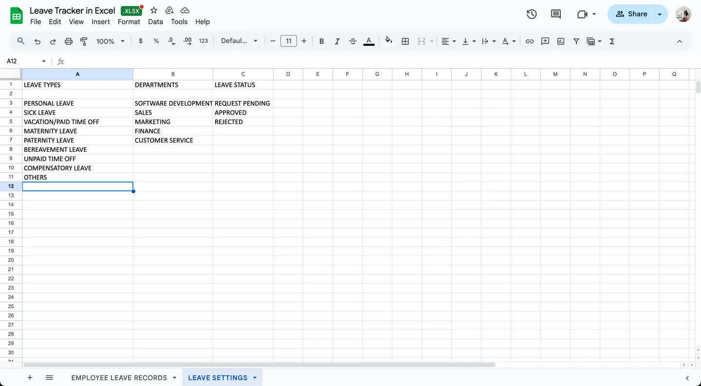
Once we have created the columns and added the list under each, we are ready to begin with the creation of drop-down menus for each of these in our Excel leave tracker!

1. Create a drop-down menu for departments.

Go to the Employee Leave Records sheet.
Select the first cell below the column for departments.
Go to the ‘Data’ tab and from the ‘Data tools’ section, select ‘Data validation’.
In the ‘Settings’ tab, select ‘List’ from the drop-down menu below ‘Allow’.
Click on the empty tab below ‘Source’.
Head to the ‘Leave settings’ sheet on the workbook and select all the cells with the various departments.
Select ‘OK’.

If we select the first cell below the ‘Departments’ in the ‘Employee Leave Records’ sheet, we will find a drop-down menu with the list of all departments created. We can pick the department for the employee to the left. To create a drop-down menu for all the cells under ‘Departments’, we can simply click on the first cell and drag it to the bottom of the list.

2. Create a drop-down menu for leave types.

Go to the Employee Leave Records sheet.
Select the first cell below the column for leave types.
Go to the ‘Data’ tab and from the ‘Data tools’ section, select ‘Data validation’.
In the ‘Settings’ tab, select ‘List’ from the drop-down menu below ‘Allow’.
Click on the empty tab below ‘Source’.
Head to the ‘Leave settings’ sheet on the workbook and select all the cells with the various leave types.
Select ‘OK’.

We will now be able to see a drop-down menu for leave types by clicking the first cell below ‘Leave types’. To add a drop-down menu for all the cells under ‘Leave types’, we will simply click on the first cell and drag it to the bottom of the list.

3. Create a drop-down menu for leave status.

Go to the Employee Leave Records sheet.
Select the first cell below the column for leave status.
Go to the ‘Data’ tab and from the ‘Data tools’ section, select ‘Data validation’.
In the ‘Settings’ tab, select ‘List’ from the drop-down menu below ‘Allow’.
Click on the empty tab below ‘Source’.
Head to the ‘Leave settings’ sheet on the workbook and select all the cells with the various leave statuses.
Select ‘OK’.

On selecting the first cell under ‘Leave status’, we can now find a drop-down menu with the three options for selecting a leave status. We will now simply drag this cell to the bottom of the same column to create a drop-down menu for the rest of the cells in the column.

Step 4: Calculating total days of leave automatically

Let us now see how the total days of leave will be calculated. We will use a formula for calculating this. The formula used will be: =NETWORKDAYS(E2, F2) in the cell below ‘Total days of leave’, where E2 is the cell containing the start date of the leave requested and F2 is the cell containing the end date of the leave requested.

Here are the steps:

Write the text in the formula.
Add an open bracket.
Select the cell containing the start date of the leave requested.
Add a comma.
Select the cell containing the end date.
Add the close bracket and hit enter.

The total days of leave requested will appear in the selected cell below ‘Total days of leave’.

Step 5: Set up conditional formatting for leave status

Lastly, we will color code the options for ‘Leave status’-request pending, approved, and rejected, using conditional formatting. This will help us to easily identify the status of a leave request on our leave tracker in Excel.

We have decided to use the red color for ‘Request pending’, the green color for ‘Approved’, and the black color for ‘Rejected’.

To do this, we will follow the steps below:

Go to the ‘Home’ tab.
Select ‘Conditional formatting’.
From the drop-down menu, pick ‘New rule’.
Under ‘Select a rule type’, select ‘Format only cells that contain’.
Below ‘Format only cells with’, select ‘Specific text’.
In the tab next, select ‘Containing’.
In the tab next, type ‘Request pending’.
Click on the ‘Format’ button below.
Go to the ‘Font’ tab and select the white color.
Go to the ‘Fill’ tab and select the red color.
Click OK.
Click OK again.

We will repeat the steps for the ‘Approved’ option.

Go to the ‘Home’ tab.
Select ‘Conditional formatting’.
From the drop-down menu, pick ‘New rule’.
Under ‘Select a rule type’, select ‘Format only cells that contain’.
Below ‘Format only cells with’, select ‘Specific text’.
In the tab next, select ‘Containing’.
In the tab next, type ‘Approved’.
Click on the ‘Format’ button below.
Go to the ‘Font’ tab and select the white color.
Go to the ‘Fill’ tab and select the green color.
Click OK.
Click OK again.

We will do the same now for the ‘Rejected’ option.

Go to the ‘Home’ tab.
Select ‘Conditional formatting’.
From the drop-down menu, pick ‘New rule’.
Under ‘Select a rule type’, select ‘Format only cells that contain’.
Below ‘Format only cells with’, select ‘Specific text’.
In the tab next, select ‘Containing’.
In the tab next, type ‘Rejected’.
Click on the ‘Format’ button below.
Go to the ‘Font’ tab and select the white color.
Go to the ‘Fill’ tab and select the black color.
Click OK.
Click OK again.

Once this is done, we will drag the selected cell below the ‘Leave status’ column to the desired last row on our employee leave tracker in Excel. You can check the drop-down menu to find the options for leave status color-coded now.

Now, we have created an employee leave tracker in Excel that we can use as and when our team members request a leave. We can simply feed in their full names and their email ID, select their department from the drop-down menu, select the leave type requested from the drop-down menu, add the start and end days of leave, calculate the days of leave requested, and finally select the status of the leave according to the action taken.

Automate leave tracking with Sup Bot

If you’re struggling with outdated PTO processes, it’s time to switch to Sup Bot. Everything happens right inside Slack, MS Teams, and Webex, saving you from managing multiple tools. Sup Bot handles everything-from automatic calculations of leave balances to syncing with Google Calendar. No more guesswork, no more manual calculations-just simple, accurate PTO tracking that keeps everyone on track. With clear access control for approvals, you decide who has the authority, making it both secure and easy. Take the hassle out of time-off management and give Sup Bot a try today.

Add to Slack

Add to Teams

Add to Webex

Frequently asked questions

1. How do I create an absence tracker in Excel?

Create an absence tracker in Excel using the following steps:

1.In the first sheet, add headings for Employee name, Employee email ID, Department, Leave type, Start date of the leave, End date of the leave, Total days of leave, and Leave status. Freeze this row.
2.Add the details for leave types, departments, and leave status in the second sheet.
3.Use data validation to create drop-downs for the department, the leave types, and the leave status.
4.Use the formula for Net Working Days.
5.Set up conditional formatting for leave statuses.

2. How to track employee leaves?

There are multiple methods for tracking employees' leaves. One option is using paper, where you create a table listing all team members and monthly dates to manually record the absences. While simple, this method is susceptible to errors. Another option is using Excel, which allows for more precise calculations but can become challenging to manage as the team grows. A more efficient approach is using a PTO tracker, such as Sup Bot, which automates the process, minimizing errors and saving time.

3. What is a leave tracker?

A PTO tracker such as the Sup Bot is a tool that companies use to manage employee leave requests more efficiently than a leave tracker in Excel. It streamlines the leave management process by preventing scheduling conflicts. The tracker also automatically calculates how many leave days each employee has remaining, saving time and reducing errors compared to manual tracking. Additionally, it provides a clear view of who is on leave on any given day, making it easier for managers and team members to plan work and coordinate tasks.

4. How to calculate absent days in Excel?

Calculate the days of absence in Excel using the following steps:

1.Add the start date and the end date of the leave request in separate cells along the same row for an individual team member.
2.In the designated cell for calculating the days of absence, write this formula: =NETWORKDAYS( B2,C2), where B2 is the cell containing data for the start date and C2 is the cell containing data for the end date.
3.To input the cell numbers in the formula, you can either write their numbers or click on them.
4.Press enter.

5. How do I record leave days in Excel?

To record leave days in Excel:

1.Set up the leave tracker in Excel using the steps mentioned above.
2.Add the name of the team member and the dates of leave requested.
3.Select the department of the team member and the requested leave type from the respective drop-down menus.
4.Calculate the days of leave using the formula: =NETWORKDAYS( E2,F2), where E2 is the cell containing the start date and F2 is the cell containing the end date.
5.Approve or reject the leave request by selecting the required option from the drop-down menu for leave status.